Using the Backoffice UI¶

The backoffice is Kaval.AI’s management and monitoring interface — a FastAPI service (kavalai.backoffice) backed by PostgreSQL or SQLite, with an Angular front end. While the SDK runs your agents, the backoffice is where they are configured, inspected and observed: every session, run, node and model call a workflow produces is recorded and browsable here. It is the visual side of Kaval.AI’s observable pillar.

The backoffice reads two databases, and never the same one twice. Its own schema holds projects, users and memberships; each project it manages points at an agent database, which is where the runtime writes. The separation is deliberate: an agent database can be handed to the backoffice read-mostly, and several environments — local, staging, production — can be inspected from one interface without their runtime data ever meeting.

Running the backoffice¶

Three things must exist before the interface is usable: a database carrying both schemas, a Google OAuth client for sign-in, and one user row to sign in as. They are treated in that order below. PostgreSQL is the production choice; SQLite serves a single machine, as described at the end of this section.

Setting up PostgreSQL¶

The repository’s docker-compose.yml provides an instance with the pgvector extension already present, which the RAG tables require:

docker compose up -d postgres_db

It exposes PostgreSQL on host port 6543 with the development credentials kavalai_dev / kavalai_dev and a database of the same name, storing its data under local_data/pgdata.

An existing PostgreSQL server (version 13 or later) serves equally well. Only a database and a role permitted to create an extension are needed:

CREATE DATABASE kavalai;

Then, connected to that database:

CREATE EXTENSION IF NOT EXISTS vector;

The schemas themselves need not be created by hand. Each migration set issues CREATE SCHEMA IF NOT EXISTS for its target before it runs, and the agents set creates the vector extension as its first revision:

# The backoffice's own tables: projects, users, memberships, caches.
python -m kavalai.migrate_db backoffice

# The agent runtime tables the backoffice reads: sessions, runs, tasks,
# model call statistics.
python -m kavalai.migrate_db agents

Both are idempotent and both read their connection from the environment — KAVALAI_BO_DB_URI / KAVALAI_BO_DB_SCHEMA for the first, KAVALAI_DB_URI / KAVALAI_DB_SCHEMA for the second. The two schemas may share one instance, as they do in the development stack, or live on entirely separate servers. Every variable is listed in Configuration, and the production arrangement in Deployment.

The RAG tables — the rag_collections registry and one table per collection — belong to neither migration set. A RAG service creates them on first use, which is its default. A service constructed with provision=False issues no DDL, so that the runtime role can hold data privileges only; the registry and the collections are then created beforehand by a job running under a role with owner privileges, through ensure_registry() and create_collection(). The backoffice creates neither: its RAG explorer reads the collections that exist, and a project without any shows none.

Using SQLite instead¶

Both variables also accept a sqlite:///path URI, and the schema variables are then ignored, since SQLite has no schemas. The same two commands create the tables in the named files:

KAVALAI_BO_DB_URI=sqlite:///local_data/backoffice.db \
    python -m kavalai.migrate_db backoffice
KAVALAI_DB_URI=sqlite:///local_data/agents.db \
    python -m kavalai.migrate_db agents

An agent server started with the same KAVALAI_DB_URI writes its sessions, runs and tasks into that file, and a project of type SQLite pointing at the file shows them. This suits development, a demonstration or a laptop: the agent server and the backoffice must share a filesystem, and SQLite on a network mount is not safe for a writer, so PostgreSQL remains the choice for a deployment with more than one host.

Configuring sign-in¶

Authentication is delegated to Google OAuth; the backoffice stores no passwords. Create an OAuth client in the Google Cloud console, register {backoffice}/auth/google/callback as its authorised redirect URI, and set:

KAVALAI_BO_GOOGLE_CLIENT_ID=...
KAVALAI_BO_GOOGLE_CLIENT_SECRET=...

# Signs the session cookie. Required: there is no development fallback.
KAVALAI_BO_SESSION_SECRET_KEY=...

# Where a completed sign-in is redirected to.
KAVALAI_BO_FRONTEND_URL=http://localhost:8000

Starting the service¶

The development stack builds the image, applies the backoffice migrations and serves the interface — API and compiled front end together — at http://localhost:8000:

docker compose up postgres_db backoffice-migrations backoffice

To run it from a checkout instead, start the API and the Angular development server separately. The API binds to KAVALAI_BO_HOST / KAVALAI_BO_PORT, and the front end proxies to it, so KAVALAI_BO_FRONTEND_URL must then name the Angular port:

python -m kavalai.backoffice.server      # API, port 8000 unless set
cd frontend && npm start                 # UI on http://localhost:4200

Signing in¶

The landing page offers a single action.

Creating the first user¶

Sign-in authenticates an identity; it does not grant one. A Google account is admitted only if its address already appears in the users table — an unknown address is refused with 403 User not registered in the system and the attempt is logged. Nothing self-registers, which is why an installation that has just been migrated cannot yet be entered by anyone.

The first user is therefore inserted by hand, once, directly into the backoffice schema. Make it an administrator: only administrators may create projects and further users.

INSERT INTO backoffice.users (id, email, name, is_admin, created_at, updated_at)
VALUES (gen_random_uuid(), 'you@example.com', 'Your Name', true, now(), now());

The address must match the Google account exactly; name and picture are overwritten from the Google profile on every sign-in, so their initial values matter little. Against the development stack the statement can be applied with:

docker compose exec postgres_db \
  psql -U kavalai_dev -d kavalai_dev -c "INSERT INTO backoffice.users \
  (id, email, name, is_admin, created_at, updated_at) VALUES \
  (gen_random_uuid(), 'you@example.com', 'Your Name', true, now(), now());"

This is the only step that requires database access. Once that account can sign in, every further user is added from the Users page and every project from the interface itself.

Projects¶

Everything in the backoffice is scoped to a project. A project carries a name, a description, the connection details of its agent database, its members, and a cache in which derived artefacts such as trained PCA models are kept. The Database Type selects how the connection is described: a PostgreSQL project names host, port, user, password, database and schema; a SQLite project names the database file, which the backoffice must be able to read from its own filesystem. A PostgreSQL project may also name a RAG Schema, for a deployment that keeps its RAG collections in a schema of their own beside the runtime tables; left empty, the collections are looked for in the schema above. The project page is where the active project is chosen, new ones are created, and the connection is verified.

Read-only is on for every project unless switched off. The backoffice only reads an agent database, and the database it is pointed at may be production, so the guarantee is placed where it cannot be argued with: every connection a read-only project opens is set to refuse writes by the database itself — default_transaction_read_only on PostgreSQL, PRAGMA query_only on SQLite — whatever the connecting role would otherwise be allowed to do, and the RAG explorer’s service never creates a registry or a collection. A project can be switched to read-write, which changes nothing today, since no page writes; the switch exists so that a future page that must write cannot do so on a project nobody opened for it.

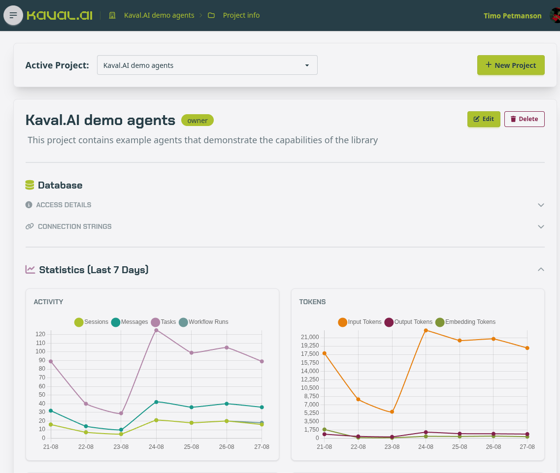
The Statistics (Last 7 Days) panels are read from the agent database rather than from the backoffice’s own: sessions, messages, tasks and workflow runs on the left, input, output and embedding tokens on the right. They are the first indication that a project’s connection is sound and that the runtime is in fact writing to the schema the project names.

The selected project follows the user across pages, and is stored as active_project_id. If the project is later deleted, or the membership revoked, that value is re-resolved on the next page load rather than left to answer 403 — a session that goes stale repairs itself without a re-login.

Agents¶

The Agents page lists the agents that have written to the active project’s database. Selecting one renders its workflow as a graph — the same renderer the documentation uses, so the picture in the interface and the picture in Workflows are produced by one code path — alongside the declared Input and Output models and the agent’s headline counters.

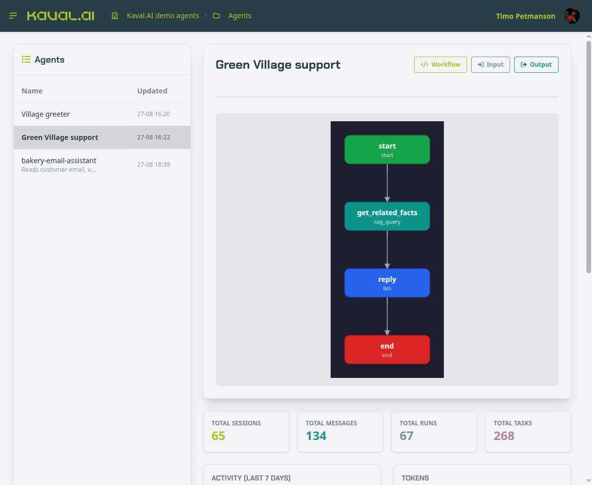
The graph is the workflow as the engine parsed it, not as it was written: node names carry their type beneath them — rag_query, llm, start, end — so a definition can be checked against what is actually being served.

The counters below it (total sessions, messages, runs and tasks) and the seven-day charts describe one agent rather than the whole project, which makes this the quickest view for judging how heavily a single agent is used.

Workflow monitoring¶

The Workflows page is a monitoring timeline: one row per agent, one marker per recent run. Completed runs are filled and empty runs are flagged, which gives an at-a-glance health view across every agent in the project and a route into any individual run.

Conversations¶

A conversation is a session: the runs triggered within it, the messages exchanged, and the errors raised. The list is filtered by agent, by date range, and by external identifier — the last of these is how evaluation runs are found, since Evaluation & acceptance testing records each case under eval:{tag}:{case}.

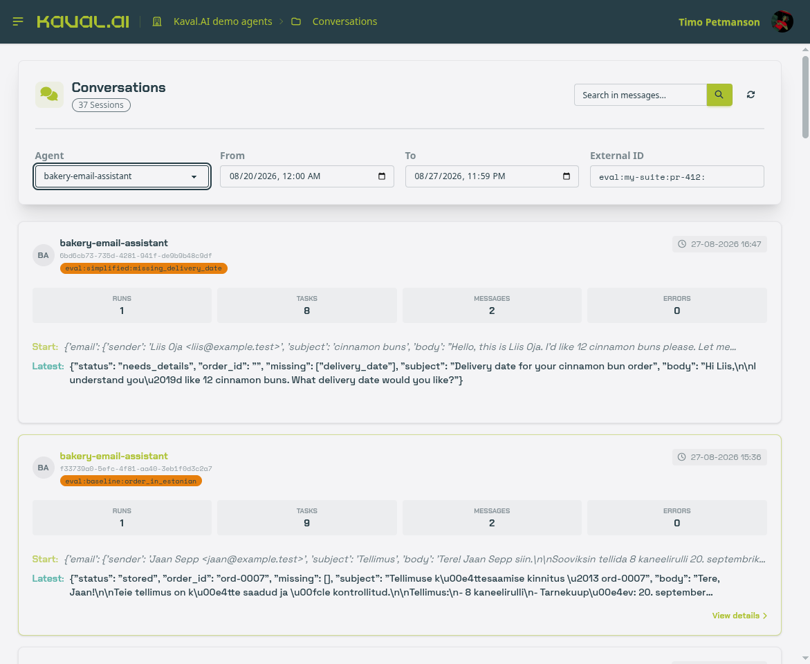
Each entry shows the counts for that session and, below them, its first and latest payloads. Because a Kaval.AI workflow’s boundaries are typed, those payloads are structured data rather than prose: in the illustration the bakery assistant’s latest output carries status, order_id and missing beside the human-readable subject and body, so what the workflow decided is legible without reading what it wrote.

The list is ordered by last activity — the time of a session’s most recent run — and that is the time each entry shows. A conversation resumed today therefore stands above one begun today and left idle since. The date range, by contrast, filters on the time a session was created.

The task debugger¶

Opening a conversation descends one further level, to the runs it contains and the tasks each run executed. A run names its nodes in execution order, and every node can be opened on its own.

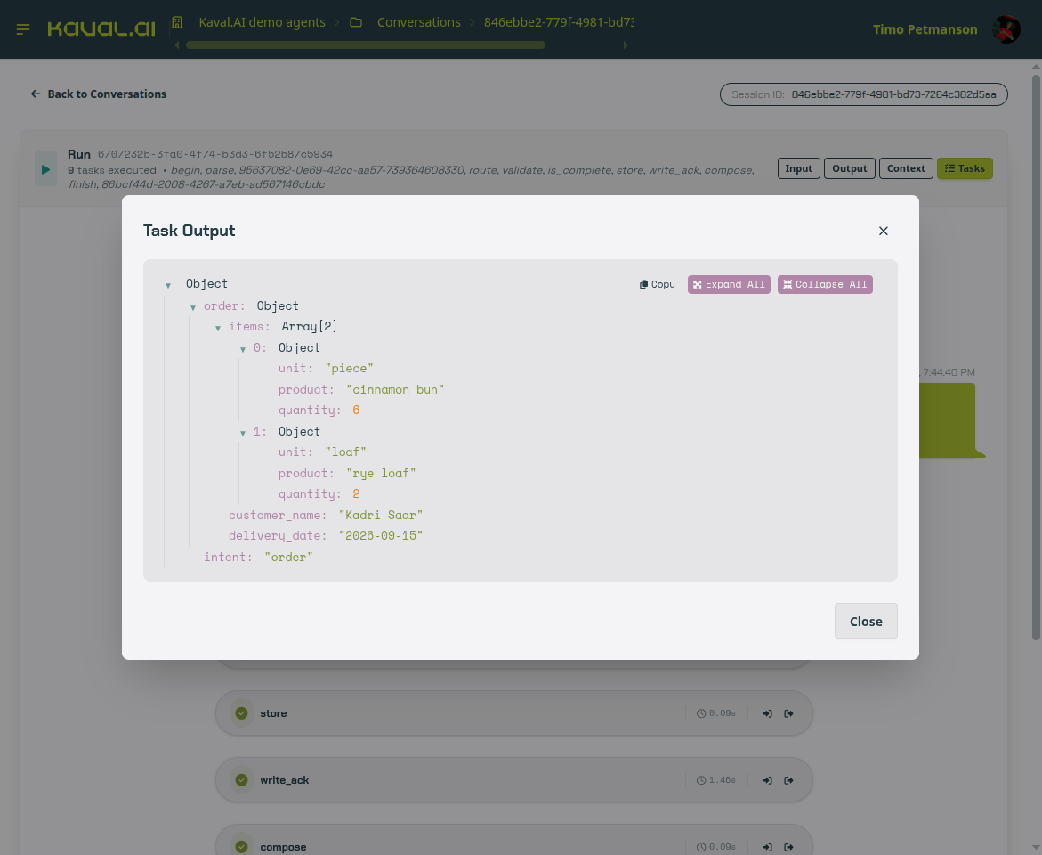
Each task records its duration and its status, and exposes the value that entered it and the value that left it. The output opens in an expandable viewer: here the parse node’s result is the order it extracted from a customer’s email — two items with product, quantity and unit, a customer name, a delivery date and the intent it classified. The Input, Output and Context buttons at run level show the same for the run as a whole.

A rag_query node records its retrieval in the same place. Its inputs name the query, the collection, top_k, source_ids and min_similarity; with store: content its output holds the joined passage text as content and, as hits, the identifier, source identifier, similarity and metadata of each passage, so a retrieval can be judged from the task without running the query again.

The run’s context also carries the per-run template values a caller passed, as run_templates, since a prompt cannot be explained without them. A failed run is recorded too: its context holds status and error and, unless the engine was created with record_context=False, the data the run had reached.

Beneath the tasks, Model Calls lists the model calls the run made, oldest first — model, call type, input, output and total tokens, and duration — with the run’s token total and a link to the same calls on the Model calls page. The embedding calls of the run’s rag_query nodes are among them. The section shows the hundred most recent calls, and is absent when the run made none.

This is the intended way to answer “why did it do that”: each node’s own input and output are stored, so a wrong answer can be traced to the step that first went wrong rather than inferred from the final reply. The rows come from the task-logger backend described in Observability, and are written only when a workflow is run with one configured.

Model calls¶

The Model calls page lists every LLM and embedding call the runtime made: provider and model, status, duration, prompt and completion tokens — cached prompt and reasoning tokens among them — and the request and response payloads. Each row is a ModelCallStat. There is no cost column, and deliberately so: providers report tokens rather than money, and cached input is priced differently enough that a derived total would be wrong rather than merely stale.

Each call is attributed to the run that made it: a row carries the run’s run_id and session_id, the embedding calls of a workflow’s rag_query nodes included, whose response payload records no vectors. Neither identifier is a foreign key, so the token counts outlive the conversation they belong to. A card links to its conversation and to the run’s tasks, and its run identifier narrows the page to that run’s calls. The same filters are the page’s run_id and session_id query parameters, which is how the Model calls button of a conversation and the task debugger reach it; Show all calls removes them.

RAG explorer¶

The RAG page is the interface’s answer to a question the SDK can only answer in a notebook: what is actually in this index, and does it retrieve what one would expect? It reads the project’s vector collections directly through the project’s RAG service — PostgresRagService or SqliteRagService, which share one storage model (see The database and data model) — so it needs no agent, no workflow and no running server — only a project whose database holds an index.

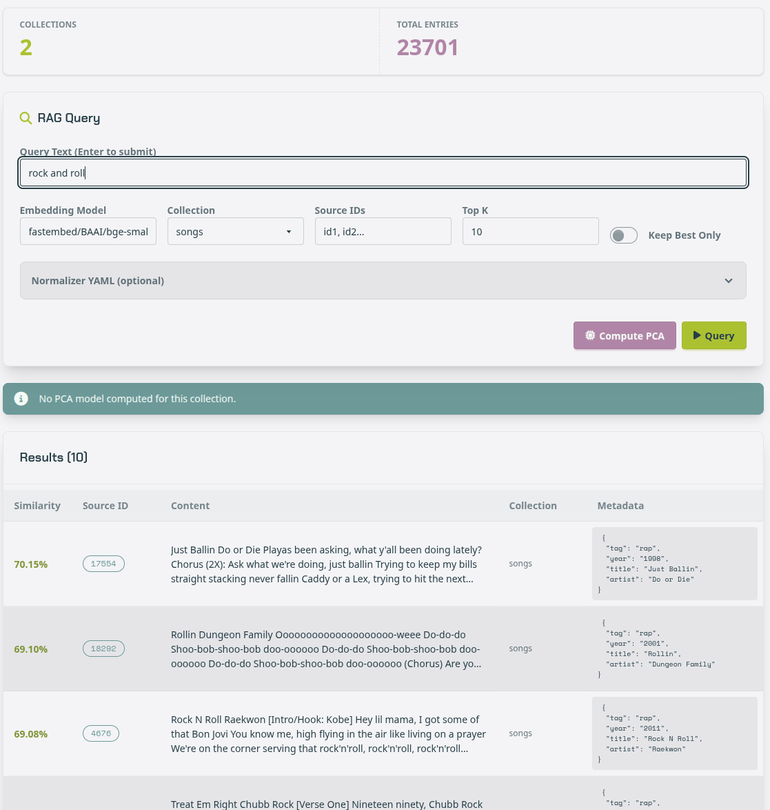
Two counters head the page — the number of collections in the database and the total number of indexed entries across them. Beneath them sits the query form, whose controls correspond one for one to the arguments of query():

Results are returned ranked by similarity, reported as higher-is-better cosine similarity (1 - distance) on every backend, so the figures are comparable across storage engines. Each row carries its source identifier, the retrieved content, its collection, and the metadata it was indexed with — the same rag_metadata a RagServiceResult exposes to a workflow. Reading a retrieval failure off this table is usually immediate: either the intended passage is absent from the index, or it is present and ranked below something else.

Projecting the embedding space¶

Similarity figures say how close a match is; they do not say what the neighbourhood looks like. Compute PCA fits a two-dimensional projection of the collection so that it can be seen.

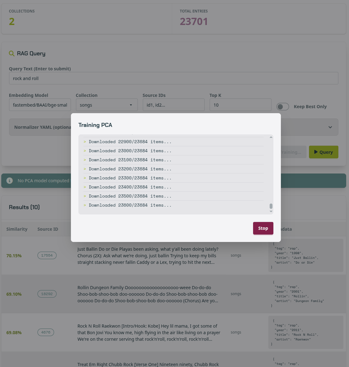
Training streams its progress over Server-Sent Events and can be stopped from the dialog. The embeddings are exported from the collection, an incremental PCA is fitted over them in batches, and both the fitted model and a sample of 500 projected points are stored in the project’s cache. The work is done once per collection: subsequent queries reuse the stored model, and a page whose collection has no model yet says so plainly rather than showing an empty plot. A query is projected from an embedding computed with the collection’s recorded model, the space in which the PCA was fitted.

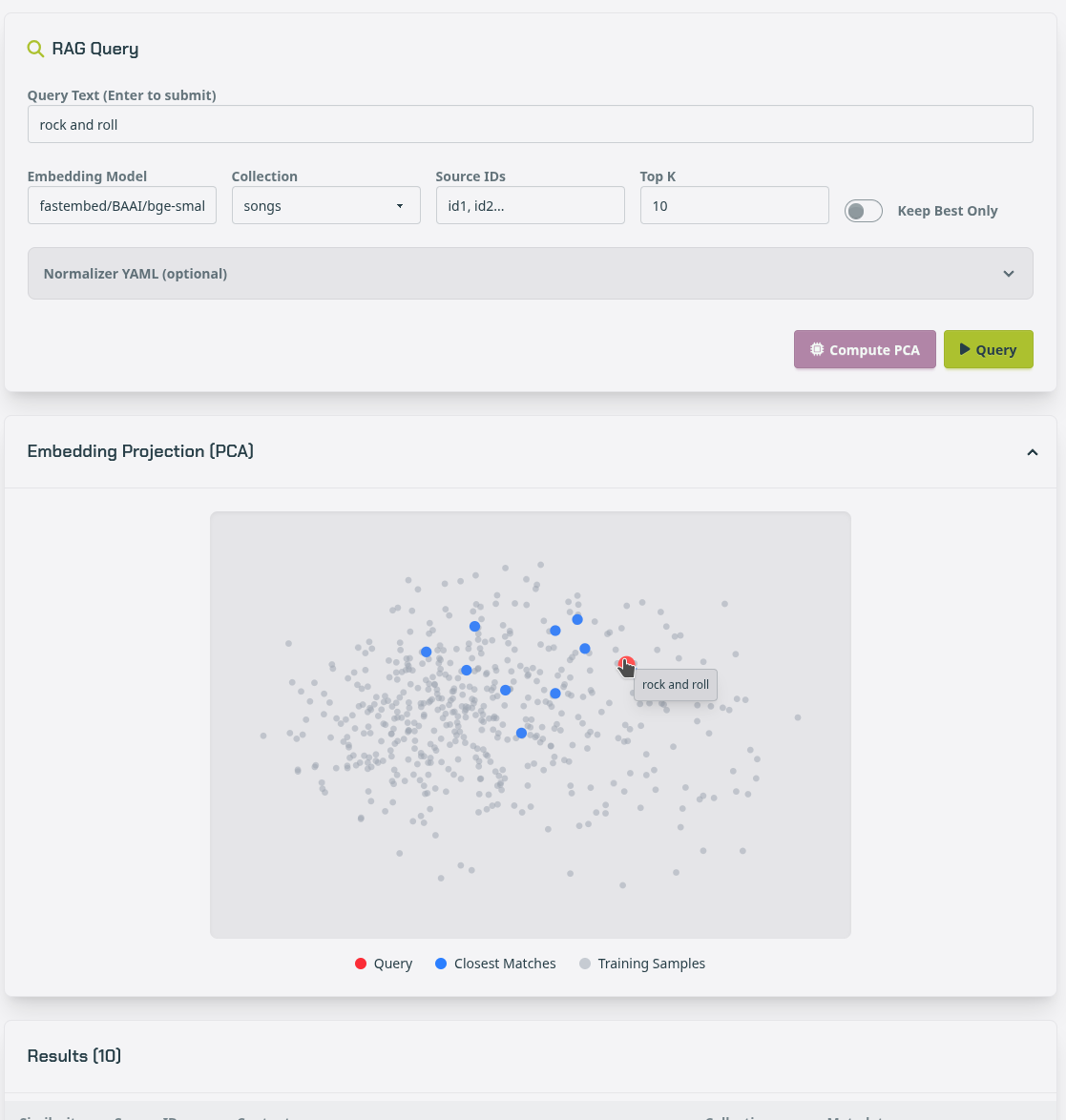
The projection then accompanies every query against that collection. The cached sample is drawn in grey as the shape of the corpus, the query in red, and its nearest neighbours in blue; hovering a point reveals what it is. Two components of a many-hundred-dimensional space are a lossy summary and should be read as one — but they answer questions a ranked list cannot. Whether the retrieved matches form a cluster or are scattered, whether the query falls inside the corpus or at its edge, and whether a collection is one body of text or several, are all visible at a glance. A query that lands far from every grey point is a query the index was never built to answer, and the similarity figures beneath it should be read in that light.

Users and access¶

The Users page is administrator-only. It is where accounts are created after the first — an address and a name, with the administrator flag granted or withheld — and where they are removed. An administrator cannot delete their own account, which prevents an installation from being locked out of itself.

Membership is granted per project, in one of two roles. A viewer may read everything the project exposes; an owner may in addition edit the project, manage its members and delete it. The last owner of a project can be neither removed nor demoted, so a project cannot be orphaned. Every project-scoped endpoint verifies membership on the server, so the interface hides only what the API would refuse in any case.